Data acquisition circuit: -
.png)
.jpeg)
This is the data acquisition circuit that we have used to amplify the weak signal from the CT sensor before taken by the microcontroller. The range of output voltages will be in the range of 2.2v to 0v. The gain of this non inverting amplifier is nearly 5 times. The output is then connected to analog pin of microcontroller board.
Experimental setup: -
.jpeg)
As part of our project, we decided to use three devices for experimentation purposes. For this, we used a table fan, phone charging and laptop charging. We had used a single-phase AC meter with voltage rating 240V, 50 Hz and current rating of 5 – 30A and it would also track the power consumed in due time. The input of meter is connected to one of the sockets in our experimental area and the output from the meter is connected to a switch board with 3 sockets having a switch for each.
Single phase ac meter
.jpeg)
A single-phase AC meter is a device used to measure electrical energy consumption in a single-phase alternating current (AC) electrical system. In single-phase systems, the power is distributed through two wires: one active (also known as "hot" or "live") wire and one neutral wire.
Ph (phase) - In single-phase electrical systems, there is one phase, which refers to the alternating current waveform that powers the electrical devices. The phase is represented by a sinusoidal waveform, where the voltage and current periodically change direction.So, when you see "Ph" in a single-phase AC meter, it's indicating that the meter is designed to measure parameters related to that single phase of the electrical system, such as voltage, current, power factor, and energy consumption.
E(energy) - The "E" on a single-phase AC meter usually indicates the measurement of electrical energy consumption. The meter accumulates the energy consumed by measuring the product of voltage, current, and time. This accumulated energy is typically represented in units such as kilowatt-hours (kWh), which is a standard unit for measuring electricity consumption. So, when you see "E" on a single-phase AC meter, it's indicating the amount of electrical energy that has been consumed over a certain period.
R(resistance)- In the context of electrical circuits connected to the meter, "R" might refer to the resistance of the load being measured. In single-phase systems, this could include the resistance of appliances, lighting, or any other electrical devices connected to the circuit.
Cal(calibration)- Calibration is the process of adjusting and verifying the accuracy of a measuring instrument, such as an AC meter, by comparing its readings to a known standard. This ensures that the meter provides accurate measurements over its operating range.
DATA COLLECTION
Basic idea: -
- As our experimental setup includes 3 devices which we would be working to try our model classify which type and what devices are on at that particular time.
- Since we have three types of devices; our data set will have 8 possible classes of data.
| Appliance A | Appliance B | Appliance C | Appliances on | Model Output | ||
| 0 | 0 | 0 | Off | Label 1 | ||
| 0 | 0 | 1 | C | Label 2 | ||
| 0 | 1 | 0 | B | Label 3 | ||
| 0 | 1 | 1 | B, C | Label 4 | ||
| 1 | 0 | 0 | A | Label 5 | ||
| 1 | 0 | 1 | A, C | Label 6 | ||
| 1 | 1 | 0 | A, B | Label 7 | ||
| 1 | 1 | 1 | on | Label 8 | ||
- Since all the devices in our experiment (even in our households) are connected in parallel – the voltage remains same throughout all the devices. The only parameter that changes for each label is the current. Therefore, we only try to figure out the variations in the ADC input that we are getting from the data acquisition circuit
- 12-bit ADC tries to collect samples from the data acquisition circuit with each sample duration of 20 seconds and sampling frequency of 100Hz.
Our approach: -
- We started collecting our samples for each class. We have considered four such classes as follows:
| fan | Phone | laptop | Label |
| off | off | off | Standby |
| off | on | on | Phone-laptop |
| on | off | off | Fan |
| off | on | off | phone |
- Each sample collected for duration of 20 seconds with sampling frequency of 100 Hz.
- The collected samples from the analog pin of our raspberry pi rp2040 was as follows:
Class: Standby
.png)
.png)
.png)
.png)
Class: Phone -Laptop
.png)
.png)
.png)
Class: Fan
.png)
.png)
.png)
.png)
Class: Phone
.png)
.png)
.png)
.png)
- Dataset:
| Each sample size | 20 seconds |
| No. of samples for each label in training set | 80 no. |
| Total sample duration for each label in training set | 26 min 40 sec |
| No. of samples for each label in test set (includes validation set also) | 20 no. |
| Total sample duration for each label in test set (includes validation set also) | 6 min 40 sec |
| Total number of samples in training set (that includes all the four classes) | 320 no. |
| Total sample duration for all the samples in training set | 1 hr 46 min 40 sec |
| Total number of samples in test set (that includes all the four classes) | 80 no. |
| Total sample duration for all the samples in training set | 26 min 40 sec |
| Total sample duration | 2 hr 13 min 20 sec |
| Train/ test split | 80% - 20% |
FEATURE EXTRACTION
- Once we have our data set ready, we need to extract those features that seems to be unique with respect to each sample from each label. These features include maximum, minimum, average etc.
- For this purpose, we used spectral analyses block and flatten block. This would help us getting the features from each sample of data that we have collected in data collection process.
- Firstly, we define the size of each window = 20 seconds with sampling rate of 100Hz.
- Spectral analysis block:
The Spectral features block extracts frequency and power characteristics of a signal. Low-pass and high-pass filters can also be applied to filter out unwanted frequencies. It is great for analysing repetitive patterns in a signal, such as movements or vibrations from an accelerometer.
Spectral analysis parameters-
1.Scaling
Scale axes: Multiplies axes by this number to scale data from the sensor
2.Filter
- Type: Type of filter to apply to the raw data (low-pass, high-pass, or none)
- Cut-off frequency: Cut-off frequency of the filter in hertz
- Order: Order of the Butterworth filter
3.Spectral power
- FFT length: The FFT size
- No. of peaks: Number of spectral power peaks to extract
- Peaks threshold: Minimum threshold to extract a peak (frequency domain normalized to [0, 1])
- Power edges: Splits the power spectral density in various buckets (V2/Hz unit)
4. Type of analysis: wavelet type
In this type, the extracted features are statistical features, crossing features and entropy features (with 14 features per layer):
[11 no.] Features: n5, n25, n75, n95, mean, median, standard deviation (std), variance (var) and root mean square (rms), kurtosis and skewness (skew) are calculated.
[2 no.] Features: Zero crossing rate (z cross) and mean crossing rate (m cross) are the times that the signal passes through the baseline (y = 0) and the average level (y = u) per unit time respectively
[1 no.] Feature: Entropy features are characteristic measure of signal complexity
All above 14 values are calculated for each Layer (including L0, the original signal)
[Inputs]: The Wavelet Decomposition level (1, 2, ...) and what type of Wavelet (bior1.3, db2, ...) to use should be defined. If for example, level 1 is chosen, L0 and L1 are used for feature calculation.
Some of the spectral features extracted for our samples are as follows:
- For class: stand by, the wavelet approximation is as shown
.png)
.png)
The features extracted from this block for this sample is as follows:
[2.8359, 0.4716, 0.4696, -2.0457, -0.7127, 0.5741, 1.9535, -0.0912, -0.0040, 1.8917, 3.5822, 1.8917, 2.4173, 27.3250, 3.4004, 0.2253, 0.2173, -3.8493, -2.3157, 0.4374, 2.9965, -0.8151, -0.8073, 2.4524, 6.0202, 2.5818, -0.2876, 6.2867]
- For class: phone - laptop, the wavelet approximation is as shown
.png)
.png)
The features extracted from this block for this sample is as follows:
[3.5152, 0.1216, 0.1216, -10.5381, -6.0586, 0.4664, 35.4166, -3.3391, -0.0089, 12.4688, 155.6252, 12.4688, 2.5916, 6.4140, 3.2381, 0.0459, 0.1077, -49.4724, -6.8070, 5.2890, 14.1817, -2.4700, -2.7573, 20.4400, 418.2093, 20.6251, -0.4358, 5.8148]
- For class: fan, the wavelet approximation is as shown
.png)
.png)
The features extracted from this block for this sample is as follows:
[3.0777, 0.4816, 0.4835, -2.6204, -0.5752, 0.7562, 2.0161, 0.0625, -0.0019, 1.8722, 3.5088, 1.8722, -0.2174, 12.1616, 4.4162, 0.0469, 0.0409, -16.6737, -9.9121, 13.1858, 17.6014, 2.4192, 1.5605, 12.0031, 144.2181, 12.1041, -0.1445, -1.3994]
- For class: phone, the wavelet approximation is as shown
.png)
The features extracted from this block for this sample is as follows:
[2.7810, 0.4207, 0.4227, -2.9509, -0.8213, 0.7231, 2.6960, -0.0246, 0.0055, 2.5171, 6.3424, 2.5172, 2.0165, 26.0124, 3.6833, 0.0828, 0.0847, -12.5654, -3.1240, 2.8284, 12.1865, -0.3368, -0.1449, 6.5887, 43.4537, 6.5903, 0.0761, 2.2495]
- The other feature extraction block that we used is flatten block:
The Flatten block performs statistical analysis on the signal. It is useful slow-moving averages like temperature data, in combination with other blocks.
Flatten parameters:
1.Scaling
Scale axes: Multiplies axes by this number
2.Method
Average: Calculates the average value for the window
Minimum: Calculates the minimum value in the window
Maximum: Calculates the maximum value in the window
Root-mean square: Calculates the RMS value of the window
Standard deviation: Calculates the standard deviation of the window
Skewness: Calculates the skewness of the window
Kurtosis: Calculates the kurtosis of the window
The Flatten block first rescales axes of the signal if value is different than 1. Then statistical analysis is performed on each window, computing between 1 and 7 features for each axis, depending on the number of selected methods.
- For class: standby, the features extracted for the below is as follows:
.png) Features = [16.1580, 0.0000, 42.0000, 16.3159, 2.2645, 1.8288, 27.0064]
Features = [16.1580, 0.0000, 42.0000, 16.3159, 2.2645, 1.8288, 27.0064]
- For class: phone- laptop, the features extracted for the below is as follows:
.png)
Features = [16.7055, 0.0000, 108.0000, 19.6414, 10.3301, 2.3636, 11.1367]
- For class: fan, the features extracted for the below is as follows:
Features = [15.9735, 0.0000, 48.0000, 18.7391, 9.7979, 0.0478, -1.4858]
- For class: phone, the features extracted for the below is as follows:
.png)
Features = [16.1360, 0.0000, 35.0000, 16.3878, 2.8617, -0.1938, 6.7124]
MODEL DESCRIPTION
- Once our feature extraction is done; now we have for 35 features for each sample of data (28 – spectral analysis and 7 – flatten block). All these features is what we use in further computations.
- Our model consists of a three-layered neural network, with its architecture defined as follows:
import tensorflow as tf
from tensorflow.keras.models import Sequential
from tensorflow.keras.layers import Dense, InputLayer, Dropout, Conv1D, Conv2D, Flatten, Reshape, MaxPooling1D, MaxPooling2D, AveragePooling2D, BatchNormalization, Permute, ReLU, Softmax
from tensorflow.keras.optimizers.legacy import Adam
EPOCHS = args.epochs or 200
LEARNING_RATE = args.learning_rate or 0.0005
# If True, non-deterministic functions (e.g. shuffling batches) are not used.
# This is False by default.
ENSURE_DETERMINISM = args.ensure_determinism
# this controls the batch size, or you can manipulate the tf.data.Dataset objects yourself
BATCH_SIZE = args.batch_size or 32
if not ENSURE_DETERMINISM:
train_dataset = train_dataset.shuffle(buffer_size=BATCH_SIZE*4)
train_dataset=train_dataset.batch(BATCH_SIZE, drop_remainder=False)
validation_dataset=validation_dataset.batch(BATCH_SIZE, drop_remainder=False)
# model architecture
model = Sequential()
model.add(Dense(64, activation='relu',
activity_regularizer=tf.keras.regularizers.l1(0.00001)))
model.add(Dense(20, activation='relu',
activity_regularizer=tf.keras.regularizers.l1(0.00001)))
model.add(Dense(10, activation='relu',
activity_regularizer=tf.keras.regularizers.l1(0.00001)))
model.add(Dense(classes, name='y_pred', activation='softmax'))
# this controls the learning rate
opt = Adam(learning_rate=LEARNING_RATE, beta_1=0.9, beta_2=0.999)
callbacks.append(BatchLoggerCallback(BATCH_SIZE,train_sample_count,epochs=EPOCHS, ensure_determinism=ENSURE_DETERMINISM))
# train the neural network
model.compile(loss='categorical_crossentropy',optimizer=opt, metrics=['accuracy'])
model.fit(train_dataset, epochs=EPOCHS, validation_data=validation_dataset, verbose=2, callbacks=callbacks)
# Use this flag to disable per-channel quantization for a model.
# This can reduce RAM usage for convolutional models, but may have
# an impact on accuracy.
disable_per_channel_quantization = False
TRAINING MODEL
- Now we have our features ready and our model is also ready now. Its time to train our model with these features.
- Training parameters are set as follows:
No. of training cycles = 200 (number of epochs to train the neural network)
Learning rate = 0.0005 (How fast the neural network learns, if the network overfits quickly, then lower the learning rate)
- The training performance checked with that of validation data set is as follows:
Accuracy of 98.4%
.jpeg)
- The model performance checked with that of test data set is as follows:
Accuracy of 100%
.jpeg)
INFERENCE STAGE
- We have achieved the best accuracy for our model and now its time to map this to our raspberry pi rp2040 board. Since our microcontroller board is 8 bits, we need to quantize our entire model to 8 bit and also optimisation needs to be done.
- The expected hardware usage and expected accuracy by our model is as follows:
.jpeg)
- At the end we have a library ready which is compatible with Arduino ide. We used it in our code and tried to collect data from analog A0 pin continuously and output the result in real-time with a delay of around 20 seconds.
- The measured currents were as follows:
.png)
The above table shows the current that we have checked manually which would be later automated in further improvement of this project. All the above mention currents are in A(ampere) and the first value in each sub class is the status of the appliance and second one refers to the current flowing through that device.
ADAPTABILITY
- This could be scaled up to our household appliance monitoring like fridge, fan, bulb and so on. Since we had constraints with respect to the appliance that we could use, we had to restrict to small current devices.
- We had used the curated dataset from opensource to scale this to a bit bigger extent and these details are summarized as follows:
- Appliances considered are: bulb, fan, microwave, refrigerator and TV
- Data collection
The signatures of devices are taken as data from the appropriate sensors.
Bulb: -
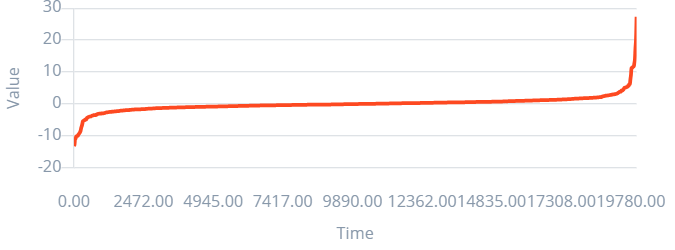
Fan: -
.png)
Microwave oven: -
Refrigerators: -
.png)
TV: -
.png)
Bulb-refrigerator: -
.png) Refrigerator – fan: -
Refrigerator – fan: -
.png)
- Feature extraction
Feature extraction blocks used are as follows:
spectral analysis
flatten
raw data
- Model architecture
This model comprises of two layered neural networks, each of 64 neurons and 8 neurons. This is defined as follows:
import tensorflow as tf
from tensorflow.keras.models import Sequential
from tensorflow.keras.layers import Dense, InputLayer, Dropout, Conv1D, Conv2D, Flatten, Reshape, MaxPooling1D, MaxPooling2D, AveragePooling2D, BatchNormalization, Permute, ReLU, Softmax
from tensorflow.keras.optimizers.legacy import Adam
EPOCHS = args.epochs or 30
LEARNING_RATE = args.learning_rate or 0.0001
# If True, non-deterministic functions (e.g. shuffling batches) are not used.
# This is False by default.
ENSURE_DETERMINISM = args.ensure_determinism
# this controls the batch size, or you can manipulate the tf.data.Dataset objects yourself
BATCH_SIZE = args.batch_size or 32
if not ENSURE_DETERMINISM:
train_dataset = train_dataset.shuffle(buffer_size=BATCH_SIZE*4)
train_dataset=train_dataset.batch(BATCH_SIZE, drop_remainder=False)
validation_dataset = validation_dataset.batch(BATCH_SIZE, drop_remainder=False)
# model architecture
model = Sequential()
model.add(Flatten())
model.add(Dense(64, activation='relu',
activity_regularizer=tf.keras.regularizers.l1(0.00001)))
model.add(Dense(8, activation='relu',
activity_regularizer=tf.keras.regularizers.l1(0.00001)))
model.add(Dense(classes, name='y_pred', activation='softmax'))
# this controls the learning rate
opt = Adam(learning_rate=LEARNING_RATE, beta_1=0.9, beta_2=0.999)
callbacks.append(BatchLoggerCallback(BATCH_SIZE, train_sample_count, epochs=EPOCHS, ensure_determinism=ENSURE_DETERMINISM))
# train the neural network
model.compile(loss='categorical_crossentropy', optimizer=opt, metrics=['accuracy'])
model.fit(train_dataset, epochs=EPOCHS, validation_data=validation_dataset, verbose=2, callbacks=callbacks)
# Use this flag to disable per-channel quantization for a model.
# This can reduce RAM usage for convolutional models, but may have
# an impact on accuracy.
disable_per_channel_quantization = False
- Accuracy (87.0%) with the validation set is found out to be as follows:
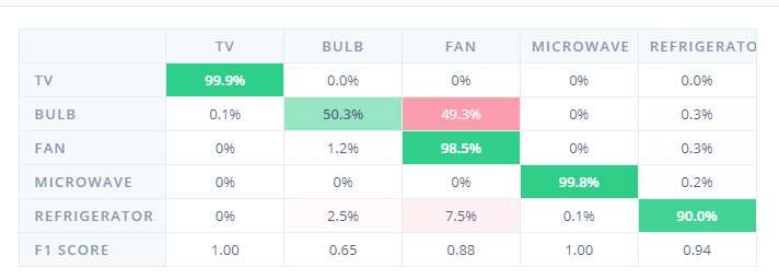
- Accuracy (87.07 %) with the test set is found to be as follows:
.jpeg)